The Haar functions
The family of N Haar functions
![]() are defined
on the interval
are defined
on the interval ![]() . The shape of the specific function
. The shape of the specific function ![]() of a given index
of a given index ![]() depends on two parameters
depends on two parameters ![]() t and
t and ![]() :
:
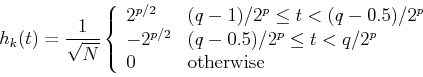
From the definition, it can be seen that ![]() determines the amplitude and
width of the non-zero part of the function, while
determines the amplitude and
width of the non-zero part of the function, while ![]() determines the
position of the non-zero part of the function.
determines the
position of the non-zero part of the function.
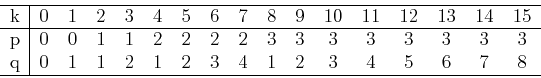
The Haar Transform Matrix
The N Haar functions can be sampled at ![]() , where
, where
![]() to
form an
to
form an ![]() by
by ![]() matrix for discrete Haar transform. For example, when
matrix for discrete Haar transform. For example, when ![]() ,
we have
,
we have
![\begin{displaymath}{\bf H}_2=\frac{1}{\sqrt{2}}\left[ \begin{array}{cc} 1 & 1 \\
1 & -1 \end{array} \right] \end{displaymath}](img23.png)
![\begin{displaymath}{\bf H}_4=\frac{1}{2}\left[ \begin{array}{cccc}
1 & 1 & 1 & 1...
...} & 0 & 0 \\
0 & 0 & \sqrt{2} & -\sqrt{2} \end{array} \right] \end{displaymath}](img25.png)
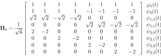
We see that all Haar functions
![]() contains a single prototype
shape composed of a square wave and its negative version, and the parameters
contains a single prototype
shape composed of a square wave and its negative version, and the parameters
The Haar transform matrix is real and orthogonal:
![\begin{displaymath}{\bf H}_4^{-1}{\bf H}_4={\bf H}_4^T {\bf H}_4=
\frac{1}{4}\le...
...& 0 & 0 0 & 0 & 1 & 0 \\
0 & 0 & 0 & 1 \end{array} \right] \end{displaymath}](img31.png)
![\begin{displaymath}{\bf H}=\left[ \begin{array}{c}
{\bf h}^T_0 {\bf h}^T_1 ...
...;\;\; {\bf H}^{-1}={\bf H}^T=[{\bf h_0},\cdots, {\bf h_{N-1}}]
\end{displaymath}](img32.png)
![\begin{displaymath}{\bf x}={\bf H}^{-1} {\bf X}={\bf H}^T {\bf X}=[{\bf h_0},\cd...
...\\ X[N-1]\end{array} \right]
=\sum_{n=0}^{N-1} X[n] {\bf h}_n \end{displaymath}](img40.png)
Comparing this Haar transform matrix with all transform matrices previously
discussed (e.g., Fourier transform, cosine transform, Walsh-Hadamard
transform), we see an essential difference. The row vectors of all previous
trnasform methods represent different frequency (or sequency) components,
including zero frequency or the average or DC component (first row ![]() ),
and the progressively higher frequencies (sequencies) in the subsequent
rows (
),
and the progressively higher frequencies (sequencies) in the subsequent
rows (
![]() ). However, the row vectors in Haar transform matrix
represent progressively smaller scales (narrower width of the square waves)
and their different positions. It is the capability to represent different
positions as well as different scales (corresponding different frequencies)
that distinguish Haar transform from the previous transforms. This capability
is also the main advantage of wavelet transform over other orthogonal transforms.
). However, the row vectors in Haar transform matrix
represent progressively smaller scales (narrower width of the square waves)
and their different positions. It is the capability to represent different
positions as well as different scales (corresponding different frequencies)
that distinguish Haar transform from the previous transforms. This capability
is also the main advantage of wavelet transform over other orthogonal transforms.
A Haar Transform Example:
The Haar transform coefficients of a ![]() -point signal
-point signal
![]() can be found as
can be found as
![\begin{displaymath}
\frac{1}{2}\left[ \begin{array}{cccc} 1 & 1 & 1 & 1 1 & 1...
...y}{c} 5 -2 -1/\sqrt{2} -1/\sqrt{2} \end{array} \right]
\end{displaymath}](img44.png)
The inverse transform will express the signal as the linear combination of
the basis functions:
![$\displaystyle \frac{1}{2}\left[ \begin{array}{rrrr} 1 & 1 & \sqrt{2} & 0 \\
1 ...
...t[ \begin{array}{c} 5 -2 -1/\sqrt{2} -1/\sqrt{2} \end{array} \right]$](img45.png) |
|||
![$\displaystyle \frac{1}{2}[5 \left[ \begin{array}{r} 1 1 1 1 \end{arra...
...ray} \right]]
= \left[ \begin{array}{r} 1 2 3 4 \end{array} \right]$](img47.png) |