Linear Models for Binary Classification

We first consider binary classification based on the same linear model $y=f({\bf x})+r={\bf x}^T{\bf w}+r$ used in linear regression considered before. Any test sample ${\bf x}$ is classified into one of the two classes $\{C_0,\,C_1\}$ depending on whether $f({\bf x})$ is greater or smaller than zero:

$$\;\;f({\bf x})={\bf w}^T{\bf x}\left\{\begin{array}{l}<0\\ >0 \end{array}\right.,\;\;\;\;\;\;\; \;\;\;\; {\bf x}\in \left\{\begin{array}{c} C_0 \\ C_1\end{array}\right.$$ (275)

Here ${\bf w}$ is a model parameter to be determined based on the training set ${\cal D}=\{({\bf x}_n,\,y_n)\vert n=1,\cdots,N\}=\{{\bf X},{\bf y}\}$, where ${\bf X}=[{\bf x}_1,\cdots,{\bf x}_N]$, ${\bf y}=[ y_1,\cdots,y_N]^T$, ${\bf x}_n\in C_n$ if $y_n=1$ and ${\bf x}_i\in C_0$ if $y_i=-1$, so that ${\bf w}$ fits all data points optimally in certain sense.

While in the previously considered least square classification method, we find the optimal ${\bf w}$ that minimizes the squared error $\varepsilon({\bf w})=\vert\vert{\bf r}\vert\vert^2$, here we find the optimal ${\bf w}$ based on a probabilistic model. Specifically, we now convert the linear function $f({\bf x})={\bf x}^T{\bf w}$ into the probability for ${\bf x}$ to belong to either class:

$$p({\bf x}\in C_1\vert{\bf w}) = p(y=1\vert{\bf x},{\bf w})$$

$$p({\bf x}\in C_0\vert{\bf w}) = p(y=-1\vert{\bf x},{\bf w}) =1-p(y=1\vert{\bf x},{\bf w})$$ (276)

This is done by a sigmoid function defined as either a logistic or cumulative Gaussian (error function, erf):

$$\;\;\;\; \sigma(z)= \frac{1}{1+e^{-z}}=\frac{e^z}{1+e^z}$$

$$\;\;\;\; \phi(z)= \int_{-\infty}^z {\cal N}(u\vert,1)\,du =\frac{1}{\sqrt{2\pi}} \int_{-\infty}^z \exp\left(-\frac{1}{2} u^2\right)\,du$$ (277)

In either case, we have

$$\sigma(z)=\left\{\begin{array}{ll}0 & z=-\infty\\ 1 & z=\infty\end{array}\right. \;\;\;\;\;\;\; \;\;\;\;\;\;\sigma(-z)=1-\sigma(z)$$ (278)

Using this sigmoid function, $f={\bf x}^T{\bf w}$ in the range of $(-\infty,\;\infty)$ is mapped to $\sigma(f({\bf x}))$ in the range of $(0,\;1)$, which can be used as the probability for ${\bf x}$ to belong to either class:

$$p(y=1\vert{\bf x},{\bf w}) = \sigma({\bf x}^T{\bf w})=\sigma(f)$$

$$p(y=-1\vert{\bf x},{\bf w}) = 1-p(y=1\vert{\bf x},{\bf w}) =1-\sigma(f)=\sigma(-f)$$ (279)

The two cases can be combined:

$$p(y\vert{\bf x},{\bf w})=\sigma(y\;{\bf x}^T{\bf w})=\sigma(yf), \;\;\;\; \;\;\;\; p(y\vert{\bf x},{\bf w})=\phi(y{\bf x}^T{\bf w})=\phi(yf)$$ (280)

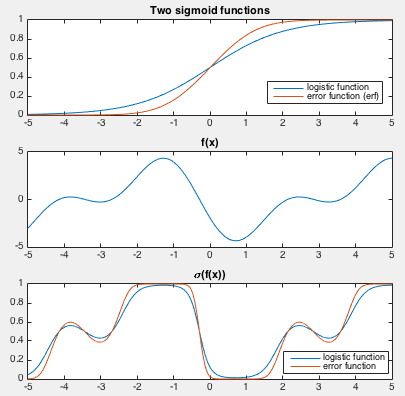
The binary classification problem can now be treated as a regression problem to find the model parameter ${\bf w}$ that best fits the data in the training set ${\cal D}=\{{\bf X},{\bf y}\}$. Such a regression problem is called logistic regression if $\sigma(z)$ is used, or probit regression if $\phi(z)$ is used.

Same as in the case of Bayesian regression, we assume the prior distribution of ${\bf w}$ to be a zero-mean Gaussian $p({\bf w})={\cal N}({\bf0},{\bf\Sigma}_w)$, and for simplicity we further assume ${\bf\Sigma}_w={\bf I}$, and find the likelihood of ${\bf w}$ based on the linear model applied to the observed data set ${\cal D}=\{({\bf x}_n,\,y_n)\vert n=1,\cdots,N\}$:

$${\cal L}({\bf w}\vert{\cal D})=p({\cal D}\vert{\bf w}) =p({\bf y}... ...f w}) =\prod_{n=1}^N \sigma(y_if_i)=\prod_{n=1}^N \sigma(y_n{\bf x}_n^T{\bf w})$$ (281)

Note that this likelihood is not Gaussian (as in the case of Eq. ()), because ${\bf y}=\pm 1$ is the binary class labeling of the training samples in ${\bf X}$, instead of a continuous function as in the case of regression.

The posterior of ${\bf w}$ can now be expressed in terms of the prior $p({\bf w})$ and the likelihood $p({\bf y}\vert{\bf X},{\bf w})$:

$$p({\bf w}\vert{\cal D}) = p({\bf w}\vert{\bf X},{\bf y}) =\frac{p({\bf y},{\bf w}\vert{\bf ... ...y}\vert{\bf X})} \propto p({\bf y}\vert{\bf X},{\bf w})\;p({\bf w}\vert{\bf X})$$

$$= \prod_{n=1}^Np(y_n\vert{\bf x}_n,{\bf w})\;{\cal N}({\bf0},{\bf\S... ...}_w\vert^{1/2}} \exp\left(-\frac{1}{2}{\bf w}^T{\bf\Sigma}_w^{-1}{\bf w}\right)$$ (282)

where the denominator $p({\bf y}\vert{\bf X})=p({\cal D})$ is dropped as it is a constant independent of the variable ${\bf w}$ of interest. We can further find the log posterior denoted by $\psi({\bf w})$:

$$\psi({\bf w})=\log \;p({\bf w}\vert{\cal D}) =\sum_{n=1}^N \log \... ...1}{2}\log\vert{\bf\Sigma}_w\vert -\frac{1}{2}{\bf w}^T{\bf\Sigma}_w^{-1}{\bf w}$$ (283)

The optimal ${\bf w}$ that best fits the training set ${\cal D}=\{{\bf X},{\bf y}\}$ can now be found as the one that maximizes this posterior $p({\bf w}\vert{\cal D})$, or, equivalently, the log posterior $\psi({\bf w})$, by setting the derivative of $\psi({\bf w})$ to zero and solving the resulting equation below by Newton's method or conjugate gradient ascent method:

$${\bf g}_{\psi}({\bf w}) = \frac{d}{d{\bf w}} \left(\sum_{n=1}^N\log \sigma(y_nf_n) \right) -\frac{d}{d{\bf w}}\left(\frac{1}{2}{\bf w}^T{\bf\Sigma}_w^{-1}{\bf w}\right)$$

$$= \sum_{n=1}^N\frac{d}{d{\bf w}} \left(\log \frac{1}{1+e^{-y_n{\bf x}_n^T{\bf w}}}\right) -{\bf\Sigma}_w^{-1}{\bf w}$$

$$= \sum_{n=1}^N\frac{y_n{\bf x}_n }{1+e^{y_n{\bf x}_n^T{\bf w}}} -{\bf\Sigma}_w^{-1}{\bf w} ={\bf0}$$ (284)

Having found the optimal ${\bf w}$, we can classify any test pattern ${\bf x}_*$ in terms of the posterior of its corresponding labeling $y_*$:

$$p(y_*=1\vert{\bf x}_*,{\bf w})=\sigma({\bf x}_*^T{\bf w}) =\sigma(f({\bf x}_*))=\frac{1}{1+\exp({\bf x}_*^T{\bf w})}$$ (285)

In a multi-class case with $(C_1,\cdots,C_K)$, we can still use a vector ${\bf w}_i$ $(i=1,\cdots,K)$ to represent each class $C_i$, the direction of the class with respect to the origin in the feature space, and the inner product ${\bf x}^T{\bf w}_i$ proportional to the projection of ${\bf x}$ onto vector ${\bf w}_i$ measures the extent to which ${\bf x}$ belongs to $C_i$. Similar to the logistic function used in the two-class case, here the soflmax function defined below is used to convert $-\infty<{\bf x}^T{\bf w}_i<\infty\,(i=1,\cdots,K)$ into the probability that ${\bf x}$ belongs to $C_i$:

$$p(y\in C_i\vert{\bf x},{\bf W}) =\frac{\exp({\bf x}^T{\bf w}_i)}{... ... & {\bf x}^T{\bf w}_i=-\infty\\ 1 & {\bf x}^T{\bf w}_i=\infty\end{array}\right.$$ (286)

where ${\bf W}=[{\bf w}_1,\cdots,{\bf w}_K]$.