Geometric Interpretation of the KLT

The optimality of the KLT discussed above can be demonstrated geometrically, based on the assumption that the random vector ${\bf x}=[x_1,\cdots,x_d]^T$ has a normal probability density function:

$$p(x_1,\cdots, x_d)=p({\bf x}) ={\cal N}({\bf x}, {\bf m}_x, {\bf\... ...[ -\frac{1}{2}({\bf x}-{\bf m}_x)^T{\bf\Sigma}_x^{-1}({\bf x}-{\bf m}_x)\right]$$ (72)

with mean vector ${\bf m}_x$ and covariance matrix ${\bf\Sigma}_x$. The shape of this normal distribution in the d-dimensional space can be represented by the iso-hypersurface in the space determined by the equation

$${\cal N}({\bf x},{\bf m}_x,{\bf\Sigma}_x)=c_0$$ (73)

where $c_0$ is some constant. This equation can be converted into an equivalent equation:

$$({\bf x}-{\bf m}_x)^T {\bf\Sigma}_x^{-1} ({\bf x}-{\bf m}_x) = c_1$$ (74)

where $c_1$ is another constant related to $c_0$. As ${\bf\Sigma}^{-1}$ is positive definite as well as ${\bf\Sigma}$, this equation represents an hyper ellipsoid in the d-dimensional space. In particular, when $d=2$, ${\bf x}=[x_1,\,x_2]^T$, with positive definite ${\bf\Sigma}_x^{-1}$:

$${\bf\Sigma}_x^{-1}=\left[ \begin{array}{cc} A & B/2 \\ B/2 & C \end{array} \right] \;\;\;\;\;\; \;\;\;\;\;\; \left\vert {\bf\Sigma}_x^{-1} \right\vert = AC-B^2/4 > 0$$ (75)

then the quadratic equation above becomes

$$({\bf x}-{\bf m}_x)^T {\bf\Sigma}_x^{-1} ({\bf x}-{\bf m}_x) = [x_1-\mu_{x_1}, x_2-\mu_{x_2}] \left[ \begin{array}{cc} A & B/2 \... ...ght] \left[ \begin{array}{c} x_1-\mu_{x_1} \\ x_2-\mu_{x_2} \end{array} \right]$$

$$= A(x_1-\mu_{x_1})^2+B(x_1-\mu_{x_1})(x_2-\mu_{x_2})+C(x_2-\mu_{x_2})^2 = c_1$$

representing an ellipse (instead of other quadratic curves such as hyperbola and parabola) centered at ${\bf m}_x=[\mu_1,\;\mu_2]^T$. When $d=3$, the quadratic equation represents an ellipsoid. In general when $d>3$, the equation ${\cal N}({\bf x}, {\bf m}_x, {\bf\Sigma}_x)=c_0$ represents a hyper-ellipsoid in the d-dimensional space.

Substituting ${\bf x}={\bf Vy}$ and ${\bf m}_x={\bf Vm}_y$ into the iso-surface equation Eq. (74), we get the equation for the hyper-ellipsoid after the KLT ${\bf y}={\bf V}^T{\bf x}$:

$$({\bf x}-{\bf m}_x)^T {\bf\Sigma}_x^{-1} ({\bf x}-{\bf m}_x) =[{\bf V}({\bf y}-{\bf m}_y)]^T{\bf\Sigma}_x{\bf V}({\bf y}-{\bf m}_y)$$

$$= ({\bf y}-{\bf m}_y)^T{\bf V}^T{\bf\Sigma}_x^{-1}{\bf V}({\bf y}-{\bf m}_y) =({\bf y}-{\bf m}_y)^T{\bf\Sigma}_y^{-1}({\bf y}-{\bf m}_y)$$

$$= ({\bf y}-{\bf m}_y)^T{\bf\Lambda}^{-1}({\bf y}-{\bf m}_y) =\sum_{... ...{y_i})^2}{\lambda_i} =\sum_{i=1}^d \frac{(y_i-\mu_{y_i})^2}{\sigma^2_{y_i}}=c_1$$ (76)

This a standardized hyper-ellipsoid. We therefore see that the KLT transform ${\bf y}={\bf V}^T{\bf x}$ is actually a rotation of the coordinate system of the d-dimensional space, which is spanned by the standard basis $\{ {\bf e}_1,\cdots,{\bf e}_d\}$ before the KLT and the eigenvectors $\{ {\bf v}_1,\cdots,{\bf v}_d\}$ as the basis vectors after the KLT.

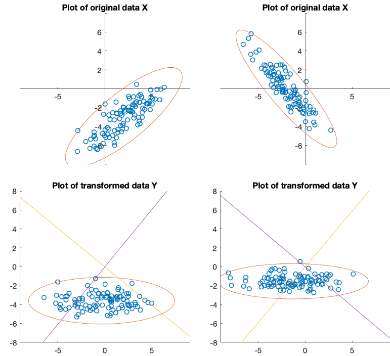
As the result, the principal semi-axes of the ellipsoid representing the Gaussian distribution of the dataset become in parallel with the axes of the new coordinate system, i.e., the ellipsoid becomes standardized. Moreover, the length of the ith principal semi-axis is proportional to the standard deviation $\sigma_{y_i}=\sqrt{\lambda_i}$ of the ith variable $y_i$. This is the reason why KLT possesses the two desirable properties: (a) the decorrelation of the signal components, and (b) redistribution and compaction of the energy or information contained in the signal, as illustrated in the figure below.

Examples