Jacobi Eigenvalue Algorithm for Symmetric Real Matrices

The Jacobi method solves the eigenvalue problem of a real symmetric matrice ${\bf A}={\bf A}^T$, of which all eigenvalues are real and all eigenvectors are orthogonal to each other (as shown here). This algorithm produces the eigenvalue matrix ${\bf\Lambda}$ and eigenvector matrix ${\bf V}$ satisfying ${\bf A}{\bf V}={\bf V}{\bf\Lambda}$.

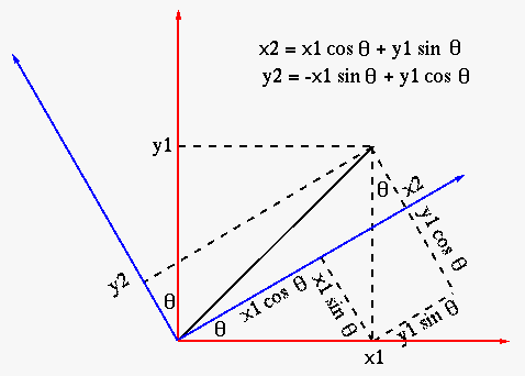
We first review the rotation of a vector in both 2 and 3-D space by an orthogonal rotation matrix. In a 2-D space, the rotation matrix is

$${\bf R}(\theta) =\left[\begin{array}{rr}\cos\theta&-\sin\theta\\ ... ...eta \end{array}\right] =\left[\begin{array}{rr}c & -s\\ s & c\end{array}\right]$$ (15)

where $\theta$ is the rotation angle, $c=\cos\theta$ and $s=\sin\theta$. This rotation matrix is orthogonal satisfying ${\bf R}^{-1}={\bf R}^T$. Pre-multiplying ${\bf R}$ to a column vector ${\bf v}_1=[x_1, y_1]^T$ we get a rotated version of the vector:

$${\bf v}_2=\left[\begin{array}{c}x_2\\ y_2\end{array}\right] ={\bf... ...nd{array}\right] =\left[\begin{array}{r}cx_1-sy_1\\ sx_1+cy_1\end{array}\right]$$ (16)

Taking transpose of the equatioin, we get the rotation of the row vector ${\bf v}_1^T=[x_1,\;y_1]$ by post-multiplying ${\bf R}^T$:

$${\bf v}^T_2=[x_2,\,y_2]=({\bf Rv}_1^T={\bf v}^T_1{\bf R}^T =[x_1\... ...\;\left[\begin{array}{rr}c&s\\ -s&c\end{array}\right] =[cx_1-sy_1\;\;sx_1+cy_1]$$ (17)

As ${\bf R}$ is an orthogonal matrix, the norms of the column or row vector is preserved, i..e., $\vert\vert{\bf v}_2\vert\vert=\vert\vert{\bf R\,v}_1\vert\vert=\vert\vert{\bf v}_1\vert\vert$. The rotation can be either clockwise if $\theta>0$ or counter clockwise if $\theta<0$.

In a 3-D space, a rotation by an angle $\theta$ around each of the three principal axes can be carried out by each of the following three rotation matrices:

$${\bf R}_x(\theta) =\left[\begin{array}{rrr}1&0&0\\ 0&c&-s\\ 0&s&c... ... R}_z(\theta) =\left[\begin{array}{rrr}c&-s&0\\ s&c&0\\ 0&0&1\end{array}\right]$$ (18)

In general, in an N-D space, the rotation around the direction of the cross-product of the ith column and the jth column ${\bf c}_i\times{\bf c}_j$ (the normal direction of the plane spanned by ${\bf c}_i$ and ${\bf c}_j$), referred to as Givens rotation, can be carried out by the following matrix:

$${\bf R}_{ij}(\theta) = \left[\begin{array}{rrrrrrr} 1&\cdots&0&\cdots&0&\cdots&0\\ \vdo... ...\cdots&0&\cdots&1\end{array}\right]\begin{array}{c}\\ i\\ \\ j\\ \\ \end{array}$$

$$\;\;\;\;\;\;\;\;\;\begin{array}{ccccccccc}&&i&&&&j&&\end{array}$$ (19)

This is an identical matrix with four of its elements modified, $r_{ii}=r_{jj}=c$ and $r_{ij}=-r_{ji}=s$. As all rows and columns are orthonormal, ${\bf R}$ is orthogonal.

The Jacobi method finds the eigenvalues of a symmetric matrix ${\bf A}$ by iteratively rotating its rows and columns in such a way that all of the off-diagonal elements are eliminated one at a time, so that eventually the resulting matrix becomes the diagonal eigenvalue matrix ${\bf\Lambda}$, and the product of all rotation matrices used in the process becomes the orthogonal eigenvector matrix ${\bf V}$. Specifically, in each iteration, we pre and post multiply ${\bf R}_{ij}(\theta)$ to ${\bf A}$, so that its ith and jth columns and rows are modified, while all other elements remain the same:

$${\bf A}'={\bf R}{\bf A}{\bf R}^T =\left[\begin{array}{ccccccc} &\... ...ots&&\vdots&&\vdots\\ &\cdots&a'_{ni}&\cdots&a'_{nj}&\cdots&\end{array}\right]$$ (20)

As ${\bf A}={\bf A}^T$ is symmetric, the resulting matrix is also symmetric:

$${\bf A}'^T=({\bf R}{\bf A}{\bf R}^T)^T={\bf R}{\bf A}^T{\bf R}^T ={\bf R}{\bf A}{\bf R}^T={\bf A}'$$ (21)

For example, the 2nd and 4th columns and rows of a $5\times 5$ matrix ${\bf A}$ are modified by ${\bf R}={\bf R}_{24}(\theta)$:

$${\bf A}'={\bf R}{\bf A}{\bf R}^T=\left[\begin{array}{ccccc} 1 & 0... ...\\ 0 & 0 & 1 & 0 & 0\\ 0 &-s & 0 & c & 0\\ 0 & 0 & 0 & 0 & 1 \end{array}\right]$$

$$= \left[\begin{array}{ccccc} a_{11} & a_{12} & a_{13} & a_{14} & a_... ...\\ 0 & 0 & 1 & 0 & 0\\ 0 &-s & 0 & c & 0\\ 0 & 0 & 0 & 0 & 1 \end{array}\right]$$

$$= \left[\begin{array}{ccccc}1 & 0 & 0 & 0 & 0\\ 0 & c & 0 & -s& 0 \... ...51} & ca_{52}-sa_{54} & a_{53} & sa_{52}+ca_{54} & a_{55}\\ \end{array}\right]$$

$$= \left[\begin{array}{ccccc} a_{11} & ca_{12}-sa_{14} & a_{13} & sa... ...51} & ca_{52}-sa_{54} & a_{53} & sa_{52}+ca_{54} & a_{55}\\ \end{array}\right]$$ (22)

We can verify that as ${\bf A}^T={\bf A}$ is symmetric, i.e., $a_{ij}=a_{ji}$, the resulting ${\bf A}'$ is also symmetric. In general, the ith and jth rows and columns are updated as shown below:

$$a'_{ii} = c^2a_{ii}-cs(a_{ij}+a_{ji})+s^2a_{jj} =c^2a_{ii}-2cs a_{ij}+s^2a_{jj}$$

$$a'_{jj} = s^2a_{ii}+cs(a_{ij}+a_{ji})+c^2a_{jj} =s^2a_{ii}+2cs a_{ij}+c^2a_{jj}$$

$$a'_{ij}=a'_{ji} = c^2a_{ij}-cs(a_{ij}+a_{ji})-s^2a_{ji} =(c^2-s^2)a_{ij}+cs(a_{ii}-a_{jj})\;\;\;\;\;\;\;(i\ne j)$$

$$a'_{ik}=a'_{ki} = c a_{ik}-s a_{jk}\;\;\;\;\;\;\;\;\;(k\ne i,\;\;k\ne j)$$

$$a'_{jk}=a'_{kj} = s a_{ik}+c a_{jk}\;\;\;\;\;\;\;\;\;(k\ne i,\;\;k\ne j)$$

$$a'_{kl} = a_{kl}\;\;\;\;\;\;\;\;\;\;\;\;\;(k,l\ne i,j)$$ (23)

As ${\bf R}$ is an orthogonal matrix that preserves the norms of the row and column vectors of ${\bf A}$, i.e., $\vert\vert{\bf a}'_i\vert\vert=\vert\vert{\bf Ra}_i\vert\vert=\vert\vert{\bf a}_i\vert\vert$, when an off-diagonal element $a_{ij}$ $(i\ne j)$ is eliminated to zero, the values of the diagonal elements $a'_{ii}$ and $a'_{jj}$ will be increased. We desire to find the rotation angle $\theta$ so that after the rotation the off-diagonal element becomes zero:

$$a'_{ij}=(c^2-s^2)a_{ij}+cs(a_{ii}-a_{jj})=0$$ (24)

This equation can be written as

$$\frac{a_{jj}-a_{ii}}{a_{ij}}=\frac{c^2-s^2}{cs}=\frac{1-(s/c)^2}{s/c} =\frac{1-t^2}{t}=2w \;\;\;\;\;\;\; \;\;\;\;\;\;t^2+2wt-1=0$$ (25)

where we have defined

$$t=\tan\theta=\frac{\sin\theta}{\cos\theta}=\frac{s}{c}, \;\;\;\;\... ...;\;\;\; w=\frac{c^2-s^2}{2cs} =\frac{\cos(2\theta)}{\sin(2\theta)}=cot(2\theta)$$ (26)

Solving the equation above for $t$, we get

$$t_{1,2}=-w\pm\sqrt{w^2+1}$$ (27)

We will always choose the root with the smaller absolute value for better precision:

$$t=\left\{\begin{array}{ll} -w+\sqrt{w^2+1}&\;\;\;\;\;\;\;\;w>0\\ -w-\sqrt{w^2+1}&\;\;\;\;\;\;\;\;w<0\end{array}\right.$$ (28)

Having found $t$, we can further find $s$ and $c$ in the rotation matrix ${\bf R}_{ij}(\theta)$:

$$s=\sin\theta=\frac{\tan\theta}{\sqrt{1+\tan^2\theta}}=\frac{t}{\s... ...;\;\;\;\;\; c=\cos\theta=\frac{1}{\sqrt{1+\tan^2\theta}}=\frac{1}{\sqrt{1+t^2}}$$ (29)

by which $a_{ij}=a_{ji}$ will be eliminated. This process is repeated to eliminate the off-diagonal component with the maximum absolute value, the pivot, until eventually the matrix becomes diagonal, containing all eigenvalues.

Note that in each iteration only the ith and jth rows and columns of the matrix are affected, we can therefore update these rows and columns alone based on the equations given above, without actually carry out the matrix multiplication to reduce computational cost.

Moreover, to minimize the roundoff error, we prefer to update the elements of the rows and columns in an iterative fashion by adding a term to its old value. To do so, we first solve the equation above $a'_{ij}=(c^2-s^2)a_{ij}+cs(a_{ii}-a_{jj})=0$ for $a_{ii}$ and $a_{jj}$ to get

$$\left\{\begin{array}{l} a_{ii}=a_{jj}-a_{ij}(c^2-s^2)/sc \\ a_{jj}=a_{ii}+a_{ij}(c^2-s^2)/sc \end{array}\right.$$

Substituting these into the expressions for $a'_{jj}$ and $a'_{ii}$ respectively, we get the following iterations:

$$a'_{jj}=s^2a_{ii}+2cs a_{ij}+c^2a_{jj} =s^2\left(a_{jj}-\frac{c^2-s^2}{sc}a_{ij}\right)+2cs a_{ij}+c^2a_{jj} =a_{jj}+t a_{ij}$$ (30)

and

$$a'_{ii}=c^2a_{ii}-2cs a_{ij}+s^2a_{jj} =c^2a_{ii}-2cs a_{ij}+s^2\left(a_{ii}+\frac{c^2-s^2}{sc}a_{ij}\right) =a_{ii}-t a_{ij}$$ (31)

We then rewrite the update equations for $a'_{ik}$ and $a'_{jk}$ as:

$$\left\{\begin{array}{l} a'_{ik}=c a_{ik}-s a_{jk}=a_{ik}+(c-1)a_{... ...ik}=a_{jk}+(c-1)a_{jk}+sa_{ik} =a_{jk}+s(a_{ik}-\tau a_{jk}) \end{array}\right.$$

where

$$\tau=\frac{1-c}{s}=\frac{s}{1+c}=\frac{1-\cos\theta}{\sin\theta} =\frac{\sin\theta}{1+\cos\theta}=\tan(\theta/2)$$ (32)

If we set an off-diagonal element to zero $a_{ij}=0$ by ${\bf R}_{ij}(\theta)$, with $c=\cos\theta$ and $s=\sin\theta$ defined above, then the values of the diagonal elements $a'_{ii}$ and $a'_{jj}$ of the resulting matrix ${\bf A}'={\bf R}^T{\bf A}{\bf R}$ will be increased. If we iteratively carry out such rotations to set the off-diagonal elements to zero one at a time

$${\bf A}''={\bf R}^T_2{\bf A}'{\bf R}_2={\bf R}^T_2{\bf R}^T_1{\bf A}{\bf R}_1{\bf R}_2$$

$$\cdots \cdots \cdots \cdots \cdots \cdots$$

$${\bf A}^{(k)}={\bf R}^T_k\cdots{\bf R}^T_1{\bf A}{\bf R}_1\cdots{\bf R}_k$$ (33)

until eventually the resulting matrix ${\bf A}^{(k)}={\bf\Lambda}$ becomes diagonal containing the eigenvalues of ${\bf A}$, and ${\bf V}={\bf R}_1\cdots,{\bf R}_k$ contains the corresponding eigenvectors.

In summary, here are the steps in each iteration of the Jacobi algorithm:

• Find the off-diagonal element $a_{ij}$ ($i\ne j$) of the greatest absolute value, the pivot, and find $w=(a_{jj}-a_{ii})/2a_{ij}$.
• Solve the quadratic equation $t^2+2wt-1=0$ for $t=\tan\theta$.
• Obtain $c=1/\sqrt{1+t^2}$ and $s=t/\sqrt{1+t^2}$.
• Update all elements in the ith and jth rows and columns.

The iteration terminates when all off-diagonal elements are close enough to zero, and we get a diagonal matrix as the eigenvalue matrix:

$${\bf V}^T{\bf A}{\bf V}={\bf\Lambda}$$ (34)

where ${\bf V}={\bf R}_1{\bf R}_2{\bf R}_3\cdots$ is the eigenvector matrix.

Example: Find the eigenvalue matrix and eigenvector matrix of the following matrix:

$${\bf A}=\left[\begin{array}{cc}3&2\\ 2&1\end{array}\right]$$

• Find $w$:

  $$w=\frac{a_{22}-a_{11}}{2a_{12}}=\frac{1-3}{4}=-\frac{1}{2}$$ (35)

• Find $t=\tan\theta$. As $w<0$, we have

  $$t=\tan\theta=-(w+\sqrt{w^2+1})=\frac{1}{2}(1-\sqrt{5})=-0.618$$ (36)

  The rotation angle is $\theta=\tan^{-1}(-0.618)=-31.7175^\circ$.
• Find $c$ and $s$

  $$c=\frac{1}{\sqrt{1+t^2}}=0.8507,\;\;\;\;\;\;s=\frac{t}{\sqrt{1+t^2}}=-0.5257$$ (37)

• Find $\lambda_1$ and $\lambda_2$

  $$\lambda_1=a'_{11}=a_{11}-t a_{12}=4.2361,\;\;\;\;\;\; \lambda_2=a'_{22}=a_{11}+t a_{12}=-0.2361$$ (38)

• Find the eigenvector and eigenvalue matrices:
  $${\bf V}=\left[\begin{array}{rr}c&s\\ -s&c\end{array}\right] =\le... ...array}\right] =\left[\begin{array}{cc}4.2361&0\\ 0&-0.2361\end{array}\right]$$