In numerical methods, it is important to know how reliable the numerical
result produced by a certain numerical algorithm is, in terms of how
sensitive it is with respect to the various perturbations caused by
the inevitable noise in the given data (e.g., observational error) and
computational errors in the system parameters (e.g., truncation error).
The algorithm can also be considered as a generic system or function with
the given data as the input and numerical result as the output. We can
therefore talk about how well or ill conditioned the system is. In
general, if a large difference in the output may be caused by a small
change in the input/system parameters, then the result is too sensitive
to the perturbations and therefore not reliable. Whether a problem is
well or ill defined (the system is well or ill behaved) can therefore
be measured based on such sensitivities:
- If a small change in the input causes a small change in the output,
the problem is well conditioned (well behaved).
- If a small change in the input can cause a large change in the output,
the problem is ill conditioned (ill behaved).
Specifically, How well or ill conditioned a problem is can be measured
quantitatively by the absolute or relative condition numbers
defined below:
- The absolute condition number
 is the upper bound
of the ratio between the change in output and change in input:
is the upper bound
of the ratio between the change in output and change in input:
 |
(1) |
- The relative condition number
 is the upper bound of the
ratio between the relative change in output and relative change in input:
is the upper bound of the
ratio between the relative change in output and relative change in input:
 |
(2) |
Here
 is the norm of any variable
  (real or complex scalar, vector, matrix, function, etc.), a real scalar
representing its “size”. In the following, we will use mostly the
2-norm
for any vector and the corresponding
spectral norm
for any matrix
(real or complex scalar, vector, matrix, function, etc.), a real scalar
representing its “size”. In the following, we will use mostly the
2-norm
for any vector and the corresponding
spectral norm
for any matrix  . Specifically, the spectral norm
 satisfies the following properties:
 |
(3) |
As the relative condition number compares the normalized changes in both
the input and output, its value is invariant to the specific units used
to measure them. The change in input can also be equivalently normalized
by the input plus change
 input + change in input as well as
input. The same is true for the change in the output.
input + change in input as well as
input. The same is true for the change in the output.
Obviously, the smaller the condition number, the better conditioned
the problem is, the less sensitive the solution is with respect to the
perturbation of the data (error, noise, approximation, etc.); and the
larger the condition number, the more ill conditioned the problem is.
In the following, we specifically consider the condition numbers
defined for some different systems.
System with single input and output variables
A system of a single input  and single output
  can be described
by a function
can be described
by a function  to be evaluated at a given input . The
condition number of the function at point is defined as the
greatest (worst case) ratio between the changes of the output and the
input:
to be evaluated at a given input . The
condition number of the function at point is defined as the
greatest (worst case) ratio between the changes of the output and the
input:
 |
(4) |
Here  is the symbol for supremum (least upper bound) and
 is the norm of the scaler variable which is either the absolute
value of if
is the norm of the scaler variable which is either the absolute
value of if
 is real or modulus of if
 is complex. Note that in general the condition number is a function of .
When the perturbation  is small, the Taylor expansion of the
function can be approximated as
is small, the Taylor expansion of the
function can be approximated as
 |
(5) |
i.e.,
 |
(6) |
Taking the absolute value or modulus on both sides, we get
 |
(7) |
where
 is the absolute
condition number. Dividing both sides by
is the absolute
condition number. Dividing both sides by
 , we get
 |
(8) |
where is the relative condition number:
 |
(9) |
The discussion above is for the task of evaluating the output
of a system as a function of the input . However, if the task is to
solve a given equation  , for the purpose of finding treated
as the output that satisfies the equation with
, for the purpose of finding treated
as the output that satisfies the equation with  treated as the
input, the problem needs to be converted into the form of evaluating the
function
treated as the
input, the problem needs to be converted into the form of evaluating the
function
 at
at  . The absolute condition number of
this function
. The absolute condition number of
this function
 is
is
![$\displaystyle \hat\kappa=\vert g'(y)\vert=\bigg\vert\frac{d}{dy}[ f^{-1}(y)]\bigg\vert
=\frac{1}{\big\vert f'(x)\big\vert}$](img32.svg) |
(10) |
which is the reciprocal of the absolute condition number  of
the corresponding evaluating problem. We therefore see that the larger
, or the smaller
of
the corresponding evaluating problem. We therefore see that the larger
, or the smaller  , the better conditioned the problem is.
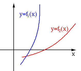
In the figure below,
 , therefore for the problem
of evaluating ,
, therefore for the problem
of evaluating ,  is more ill-conditioned than
  ,
but for the problem of solving , is better conditioned
than .
,
but for the problem of solving , is better conditioned
than .
Example: Consider the following function and its derivative:
 |
(11) |
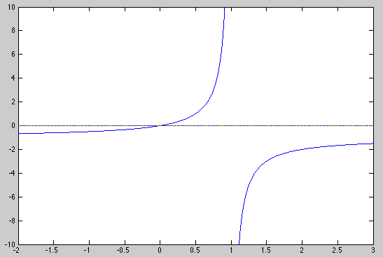
 |
(12) |
 |
(13) |
- at
 ,
,
 |
(14) |
 |
(15) |
 |
(16) |
At this point, the problem of evaluating is well-conditioned.
- at
 ,
,
 |
(17) |
 |
(18) |
 |
(19) |
At this point, the function is ill-conditioned.
We see the function is well-conditioned at but ill-conditioned
at .
However, the problem of solving the equation is very
ill-conditioned, as in the neighborhood of the root  ,
,  is very large, any value in a wide range in could result in
 , and therefore considered as a solution, which is
certainly not reliable.
, and therefore considered as a solution, which is
certainly not reliable.
Systems with Multiple input and output variables
The results above can be generalized to a system of multiple inputs
![${\bf x}=[x_1,\cdots,x_N]^T$](img52.svg) and multiple outputs
and multiple outputs
![${\bf y}=[y_1,\cdots,y_M]^T$](img53.svg) represented by a function
represented by a function
 . A change
 in the input will cause certain change in the output:
 |
(20) |
When
is small, the output can be approximated by the first
two terms of its
Taylor series expansion:
 |
(21) |
where
 is the Jacobian matrix of the function,
and we get
is the Jacobian matrix of the function,
and we get
 |
(22) |
where
is the absolute condition number defined as:
 |
(23) |
Dividing both sides of the equation above by
 we get
 |
(24) |
where is the relative condition number defined as:
 |
(25) |
In particular, consider a linear system of  inputs
and
inputs
and  outputs
described by
outputs
described by
 |
(26) |
Consider the following two problems both associated with the linear
system:
We see that both the evaluation and equation solving problems
(
 ) have the same relative condition number
 .
Let the
singular values
of be
.
Let the
singular values
of be
 ,
then the singular values of
,
then the singular values of
 are
are
 , and their
spectral norms
are their respective greatest singular values:
, and their
spectral norms
are their respective greatest singular values:
 and
and
 . Now we have
 |
(40) |
We see that the condition number of is large if its
 and
and
 are far apart in values, but it is small otherwise.
The condition number
 is a measurement of how close
is to singularity. When is singular, one or more
of its singular values are zero, i.e.,
is a measurement of how close
is to singularity. When is singular, one or more
of its singular values are zero, i.e.,
 , then
 , i.e., any problem
 associated with a singular matrix is worst conditioned. On the other
hand, as all singular values of an identity matrix
associated with a singular matrix is worst conditioned. On the other
hand, as all singular values of an identity matrix  are 1,
its condition number is
are 1,
its condition number is
 , the smallest condition
number possible, i.e., any problem
, the smallest condition
number possible, i.e., any problem
 is best
conditioned.
is best
conditioned.
In Matlab, the function cond(A,p) generates the condition number
of matrix A based on its p-norm. When  , this is the ratio between
the greatest and smallest singular values. The following Matlab commands
give the same result:
, this is the ratio between
the greatest and smallest singular values. The following Matlab commands
give the same result:
cond(A,2)
norm(A,2)*norm(inv(A),2)
s=svd(A), s(1)/s(end)
We now further consider the worst case scenarios
for both evaluating
the matrix-vector product
 and solving the
linear equation system
and solving the
linear equation system
 . In both cases, we
find
. In both cases, we
find  as the output given as the input. To do so,
we first carry out the SVD decomposition of to get
as the output given as the input. To do so,
we first carry out the SVD decomposition of to get
 with the singular values in
 sorted in descending order:
 . The inverse of can also be
SVD decomposed:
. The inverse of can also be
SVD decomposed:
 .
.
Example 1: Consider solving the linear system
 with
with
![$\displaystyle {\bf A}=\frac{1}{2}\left[\begin{array}{rr}3.0 & 2.0\\ 1.0 & 4.0\e...
...;
{\bf A}^{-1}=\left[\begin{array}{rr}0.8 & -0.4\\ -0.2 & 0.6\end{array}\right]$](img146.svg) |
(45) |
The singular values of are
 and
and
 ,
the condition number is
,
the condition number is
 |
(46) |
which is small, indicating this is a well-behaved system. Given two similar
inputs
![${\bf b}_1=[1,\;1]^T$](img150.svg) and
and
![${\bf b}_2=[0.99,\;1.01]^T$](img151.svg) with
with
![$\delta{\bf b}=[0.01,\;-0.01]^T$](img152.svg) , we find the corresponding solutions:
, we find the corresponding solutions:
![$\displaystyle {\bf x}_1={\bf A}^{-1}{\bf b}_1
=\left[\begin{array}{r}0.4 // 0.4...
...;\;\;\;\;
\delta{\bf x}=\left[\begin{array}{r}0.012 \\ -0.008\end{array}\right]$](img153.svg) |
(47) |
We have
 |
(48) |
and
 |
(49) |
Example 2:
![$\displaystyle {\bf A}=\frac{1}{2}\left[\begin{array}{rr}1.000 & 1.000\\ 1.001 &...
...\bf A}^{-1}=\left[\begin{array}{rr}-999 & 1000\\ 1001 & -1000\end{array}\right]$](img156.svg) |
(50) |
The singular values of are
 and
and
 ,
the condition number is
,
the condition number is
 |
(51) |
indicating matrix is close to singularity, and the system
is ill-conditioned. The solutions corresponding to the same two inputs
and
are
![$\displaystyle {\bf x}_1={\bf A}^{-1}{\bf b}_1
=\left[\begin{array}{r}1 \\ 1\end...
...;\;\;\;\;
\delta{\bf x}=\left[\begin{array}{r}-19.99 \\ 20.01\end{array}\right]$](img160.svg) |
(52) |
We can further find
 |
(53) |
and the condition number is:
 |
(54) |
We see that a small relative change
 in the input caused a huge change
 in
the output (2000 times greater).
in
the output (2000 times greater).
Example 3: Consider
![$\displaystyle {\bf A}=\left[ \begin{array}{ll} 3.1 & 2.0\\ 6.0 & 3.9\end{array}...
...ight]
\left[\begin{array}{rr}-0.839 & -0.544\\ -0.544 & 0.839\end{array}\right]$](img165.svg) |
(55) |
with
 |
(56) |
As is near singular, its condition number is
large, indicating that the problem associated with this
is ill-conditioned. We will now specifically consider both problems
of evaluating and solving the linear system.
Associated with whether a problem is well or ill conditioned is the
issue of an approximate solutions. For the problem of solving an
equation system
 , there exist two types
of approximate solutions:
, there exist two types
of approximate solutions:
- The approximate solution corresponds to a small residual in the
image of the function:
 |
(67) |
- The approximate solution
 is close to the true
solution
is close to the true
solution  satisfying
 (typically unknown) in the domain of the function:
 |
(68) |
If the problem is well-conditioned, the two different criteria
are consistent, i.e., the two approximations are similar,
 is small. However, if the problem
is ill-conditioned, they can be very different.
is small. However, if the problem
is ill-conditioned, they can be very different.
 .
The relative condition number of this linear system is
.
The relative condition number of this linear system is

 i.e.,
i.e.,


 for
for
 , i.e.,
  . The absolute condition
number is
. The absolute condition
number is
 .
To find the relative condition number
.
To find the relative condition number
 in the output
  in the coefficient matrix


 ,
,
 , and
, and
 .
.
 from both sides

 ,
assuming
,
assuming
 , we get


 ,
and
,
and
 .
.

 ,
,

 is the minimum right singular vector corresponding
to the smallest singular value
is the minimum right singular vector corresponding
to the smallest singular value
 . The equation
becomes:
. The equation
becomes:


![$\displaystyle {\bf A}{\bf x}=({\bf U}{\bf\Sigma}{\bf V}^*)\;{\bf v}_n
={\bf U}{...
..._n\end{array}\right]
\left[\begin{array}{c}0\\ \vdots\\ 0\\ 1\end{array}\right]$](img132.svg)
![$\displaystyle [{\bf u}_1,\cdots,{\bf u}_n]
\left[\begin{array}{c}0\\ \vdots\\ 0\\ \sigma_n\end{array}\right]
=\sigma_n{\bf u}_n$](img133.svg)

 may be
small if
may be
small if
 may be large as
 is small when
 is the maximum left singular vector corresponding
to the largest singular value
is the maximum left singular vector corresponding
to the largest singular value
 . The equation becomes:
![$\displaystyle {\bf A}^{-1}{\bf x}={\bf V}{\bf\Sigma}^{-1}{\bf U}^*{\bf u}_1
={\...
..._n\end{array}\right]
\left[\begin{array}{c}1\\ 0\\ \vdots\\ 0\end{array}\right]$](img140.svg)
![$\displaystyle [{\bf v}_1,\cdots,{\bf v}_n]
\left[\begin{array}{c}1/\sigma_1\\ 0\\ \vdots\\ 0\end{array}\right]
=\frac{1}{\sigma_1}{\bf v}_1$](img141.svg)

 may be
small if
may be
small if
 is small when
 for
for 
 .
The change in output
.
The change in output 
 times greater than any change
 and
the relative error:
and
the relative error:
![$\displaystyle {\bf x}={\bf u}_1=\left[\begin{array}{rr}-0.458\\ -0.889\end{arra...
...}={\bf A}^{-1}{\bf x}
=\left[\begin{array}{rr}-0.104\\ -0.068\end{array}\right]$](img173.svg)
![$\displaystyle \delta{\bf x}=\left[\begin{array}{rr}0.01\\ -0.01\end{array}\righ...
...f A}^{-1}\delta{\bf x}
=\left[\begin{array}{rr}0.656\\ -1.011\end{array}\right]$](img174.svg)


 .
The absolute change in output
.
The absolute change in output 
 :
:
![$\displaystyle {\bf x}={\bf v}_2=\left[\begin{array}{rr}-0.5444\\ 0.8388\end{arr...
...bf y}={\bf A}{\bf x}
=\left[\begin{array}{rr}-0.0099\\ 0.0051\end{array}\right]$](img180.svg)
![$\displaystyle \delta{\bf x}=\left[\begin{array}{rr}0.01\\ -0.01\end{array}\righ...
...y}={\bf A}\delta{\bf x}
=\left[\begin{array}{rr}0.011\\ 0.021\end{array}\right]$](img181.svg)
