SVD Transform

Let the 2D image array be represented by a matrix ${\bf A}=[ a_{ij} ]_{M\times N}$ with rank equal to $R$. Here we assume $R \leq M \leq N$. Now we consider the following eigenvalue problems for the matrix ${\bf AA}^T$ and matrix ${\bf A}^T{\bf A}$:

$${\bf AA}^T {\bf u}_i = \lambda_i {\bf u}_i,\;\;\;\;\;\; {\bf A}^T{\bf A} {\bf v}_i = \lambda_i {\bf v}_i$$

where and are M-D and N-D eigenvectors of and ${\bf A}^T{\bf A}$, respectively, and $\lambda_i,\;(i=1,2,\cdots,R)$ are the eigenvalues of both ${\bf AA}^T$ and ${\bf A}^T{\bf A}$.

Since these matrices are symmetric, their eigenvectors are orthogonal:

$${\bf u}_i^T{\bf u}_j={\bf v}_i^T{\bf v}_j=\delta_{ij}$$

and they form two orthogonal matrices ${\bf U}=[{\bf u}_1,\cdots,{\bf u}_N]_{M\times M}$ and ${\bf V}=[{\bf v}_1,\cdots,{\bf v}_N]_{N\times N}$ and

$${\bf UU}^T={\bf U}^T{\bf U}={\bf I},\;\;\;\;\;\;\;{\bf VV}^T={\bf V}^T{\bf V}={\bf I}$$

As there exist only $R$ non-zero eigenvalues, $\lambda_i > 0,\;\;(i=1,\cdots, R)$, both matrices ${\bf U}$ and ${\bf V}$ have some zero columns and the matrix ${\bf I}$ has only $R$ non-zero diagonal elements. ${\bf U}$ and ${\bf V}$ will diagonalize ${\bf AA}^T$ and ${\bf A}^T{\bf A}$ respectively:

$${\bf U}^T({\bf AA}^T){\bf U}={\bf\Lambda}_{M\times M}=diag[\lambda_1,\cdots,\lambda_R]$$

and

$${\bf V}^T({\bf A}^T{\bf A}){\bf V}={\bf\Lambda}_{N\times N} =diag[\lambda_1,\cdots,\lambda_R]$$

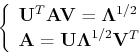
From linear algebra, we know that the singular value decomposition (SVD) of ${\bf A}$ is defined as:

$${\bf U}^T{\bf AV}={\bf\Lambda}^{1/2}=diag[\;\sqrt{\lambda_1},\cdots,\sqrt{\lambda_R}\;]$$

This can be considered as the forward SVD transform and the inverse transform can be obtained by left multiplying ${\bf U}=({\bf U}^T)^{-1}$ and right multiplying ${\bf V}^T={\bf V}^{-1}$ both sides of the equation above:

This inverse SVD transform can be so interpreted that the original image matrix is decomposed into a set of $R$ eigenimages $\sqrt{\lambda_i}[{\bf u}_i{\bf v}_i^T]$, where the outer product ${\bf u}_i{\bf v}_i^T$ is an M by N matrix.

SVD transform pair:

$$\left\{ \begin{array}{l} {\bf U}^T{\bf AV}={\bf\Lambda}^{... ...\\ {\bf A}={\bf U\Lambda}^{1/2}{\bf V}^T \end{array} \right.$$

Example: The Lenna image ${\bf A}$ together with its ${\bf U}$, ${\bf V}$ matrices and singular values ( $diag\;{\bf\Lambda}^{1/2}$):

The first 10 eigen-images of the Lenna image:

More of the eigen-images (from 10 to 120 with increment of 10):

First 10 partial sum images:

The partial sum images (from 10 to 120 eigen-images with increment 10):