Competitive learning is a typical unsupervised learning network, similar to the
statistical clustering analysis methods (k-means, Isodata). The purpose is to
discover groups/clusters composed of similar patterns represented by vectors in
the n-D space. The competitive learning network has two layers, the input layer
composed of ![]() nodes to which an input pattern
nodes to which an input pattern
![]() is
presented, and the output layer composed of
is
presented, and the output layer composed of ![]() nodes
nodes
![]() .
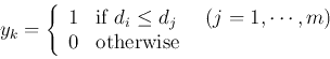
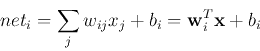
There different variations in the computation for the output, depending on the
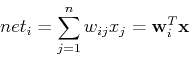
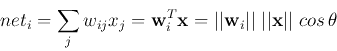
specific data and purpose. In the simplest computation, the net input, the
activation, of the ith output node is just the inner product of the weight
vector of the node and the current input vector:
.
There different variations in the computation for the output, depending on the
specific data and purpose. In the simplest computation, the net input, the
activation, of the ith output node is just the inner product of the weight
vector of the node and the current input vector:
The net input ![]() can be considered as the inner product of two vectors
can be considered as the inner product of two vectors
![]() and
and ![]() :
:
We see that the weight vector ![]() of the winning node is closest to the
current input pattern vector
of the winning node is closest to the
current input pattern vector ![]() in the n-D feature space, with smallest
angle
in the n-D feature space, with smallest
angle ![]() and therefore smallest Euclidean distance
and therefore smallest Euclidean distance
![]() .
Therefore the competition can also be carried out as:
.
Therefore the competition can also be carried out as:
The competitive learning law is

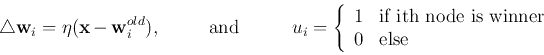
Note that
![]() is between
is between
![]() and
and ![]() ),
i.e., the effect of this learning process is to pull the weight vector
),
i.e., the effect of this learning process is to pull the weight vector
![]() closest to the current input pattern
closest to the current input pattern ![]() even closer
to
even closer
to ![]() .
.
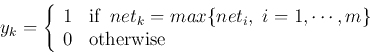
These are the main steps of the competitive learning:
Every time a randomly chosen pattern ![]() is presented to the input
layer, one of the output nodes will become the winner and it is drawn closer
to the current input
is presented to the input
layer, one of the output nodes will become the winner and it is drawn closer
to the current input ![]() . After all input patterns have been repeatedly
presented to the input layer, each group of similar patterns, a cluster in
the n-D feature space, will draw a certain weight vector to its center, and
subsequently the corresponding node will always win and produce a non-zero
output whenever any member of the cluster is presented to the input in the
future. In other words, after this unsupervised training, the n-D feature
space is partitioned into a small set of regions each corresponding to a
cluster of similar input patterns, represented by one of the output nodes,
whose weight vector
. After all input patterns have been repeatedly
presented to the input layer, each group of similar patterns, a cluster in
the n-D feature space, will draw a certain weight vector to its center, and
subsequently the corresponding node will always win and produce a non-zero
output whenever any member of the cluster is presented to the input in the
future. In other words, after this unsupervised training, the n-D feature
space is partitioned into a small set of regions each corresponding to a
cluster of similar input patterns, represented by one of the output nodes,
whose weight vector ![]() is in the central area of the region.
is in the central area of the region.
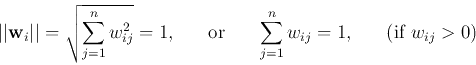
The initialization of the weight vectors may be of critical importance for the performance of the competitive learning process. It is desirable for the weight vectors to be in the same general regions as the input vectors so that all weight vectors have some opportunity to win and learn to respond to some of the input patterns. Specifically, the weight vectors can so generated that they have the same mean and covariance as the data points.
It is possible that the input patterns are not clustered into clearly
separable groups. Sometimes they even form a continuum in the feature space.
In such cases, one or a small number of output nodes may become frequent
winners of the competition while all other output nodes never win and
consequently never get the chance to learn (``dead nodes''). To prevent
such meaningless outcome from happening, a mechanism is needed that can
ensure all nodes have some chance to win. Specifically, we could modify
the learning law so that it contains an extra term:
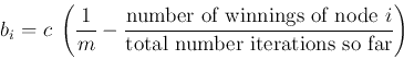
If the node is winning too often, the difference is negative thereby making it
harder for the node to win in the future. On the other hand if the node rarely
wins, the difference is positive thereby increasing its chance for the node to
win in the future. Alternatively, we can let ![]() decay by multiplying it by a
scaling factor (e.g.,
decay by multiplying it by a
scaling factor (e.g., ![]() ) each time the ith node wins. In any case, the value
of
) each time the ith node wins. In any case, the value
of ![]() needs to be fine tuned according to the specific nature of the data being
processed.
needs to be fine tuned according to the specific nature of the data being
processed.
This process of competitive learning process is also called vector quantization, by which the continuous vector space is quantized to become a set of discrete regions, called Voronoi diagram (tessellation).
Vector quantization can be used for data compression. A cluster of similar
signals ![]() in the n-D vector space can all be approximately represented
by the weight vector
in the n-D vector space can all be approximately represented
by the weight vector ![]() of one of a small number of output nodes
in the neighborhood of
of one of a small number of output nodes
in the neighborhood of ![]() , thereby the data size can be significantly
reduced.
, thereby the data size can be significantly
reduced.
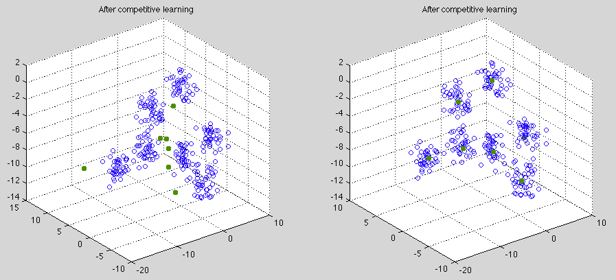
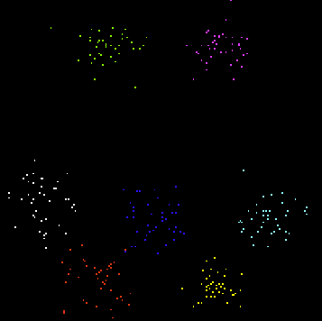
Example
As shown on the left of the figure, a set of ![]() clusters are formed by
clusters are formed by ![]() data points (blue circles) in
data points (blue circles) in ![]() dimensional space. A competitive learning network
with
dimensional space. A competitive learning network
with ![]() output nodes is then used to do clustering of the dataset. The
output nodes is then used to do clustering of the dataset. The ![]() weight
vectors (red dots) are randomly generated in the 4-D space. After competitive learning,
they moved from their initial positions (left) to the centers of the clusters (right),
thereby representing the clusters. To visualize the data points and the weight vectors
in the 4-D space is projected by the
PCA (KLT) transform
to 3-D and 2-D spaces:
weight
vectors (red dots) are randomly generated in the 4-D space. After competitive learning,
they moved from their initial positions (left) to the centers of the clusters (right),
thereby representing the clusters. To visualize the data points and the weight vectors
in the 4-D space is projected by the
PCA (KLT) transform
to 3-D and 2-D spaces:
Ideally, the number of output nodes ![]() should be the same as the number of clusters
that exist in the data set, so that each cluster of the data set can be represented
by one of the nodes after the competitive learning is complete. However, the number
of clusters in the data set is typically unknown ahead of time. In such cases, one
can carry out the competitive learning multiple times each time using a different
should be the same as the number of clusters
that exist in the data set, so that each cluster of the data set can be represented
by one of the nodes after the competitive learning is complete. However, the number
of clusters in the data set is typically unknown ahead of time. In such cases, one
can carry out the competitive learning multiple times each time using a different
![]() , and then compare the clustering results to see which
, and then compare the clustering results to see which ![]() value fits the data the
best. Specifically, how well the clustering results reflect the intrisic structure
of the data set, and, in general, the extent to which the data points are clustered,
can be quantitatively measured in terms of the scatteredness of the data point
belonging to each cluster, in comparison to the total scatteredness of the entire
dataset, as discussed
here.
Such quantitative measurement can be used as a criterion for the results of different
clustering algorithms.
value fits the data the
best. Specifically, how well the clustering results reflect the intrisic structure
of the data set, and, in general, the extent to which the data points are clustered,
can be quantitatively measured in terms of the scatteredness of the data point
belonging to each cluster, in comparison to the total scatteredness of the entire
dataset, as discussed
here.
Such quantitative measurement can be used as a criterion for the results of different
clustering algorithms.