KLT of images

A set of $N$ images of $r$ rows and $c$ columns and $K=r\times c$ pixels can be represented as a K-D vector by concatenating its $c$ columns (or its $r$ rows), and the $N$ images can be represented by a $K\times N$ array ${\bf X}$ with each column for one of the $N$ images:

$${\bf X}_{K\times N} =[{\bf x}_{c_1},\cdots,{\bf x}_{c_N}] ... ... ({\bf X}^T)_{N\times K}=[{\bf x}_{r_1},\cdots,{\bf x}_{r_K}]$$

where ${\bf x}_c_i$ is a K-D column vector containing the $K$ pixels of the ith image obtained by concatinating its columns or rows, and ${\bf x}_r_j^T$ is an N-D row vector containing the pixels at the same position of all $N$ images. If ${\bf X}$ is not degenerate, its rank is

$$R=Rank({\bf X})=\min(N,K)$$

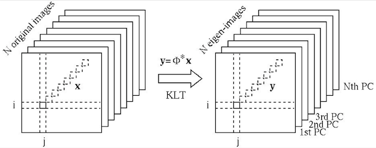
A KLT can be applied to either the column or row vectors of the data array ${\bf X}$, depending on whether the column or row vectors are treated as the realizations (samples) of a random vector.

• If the rows ${\bf x}_{r_i}$ ($i=1,\cdots,K$) of ${\bf X}$ are treated as $K$ realizations of an N-D random vector ${\bf x}_r$ (assumed to have zero mean without loss of generality), its covariance matrix can be estimated by:
  
  $${\bf\Sigma}_r=\frac{1}{K}\sum_{i=1}^K{\bf x}_{r_i}{\bf x}^T... ...x}_{r_K}^T\end{array}\right] =\frac{1}{K} ({\bf X}^T{\bf X})$$
  
  
  This is an $N \times N$ symmetric and positive semi-definite matrix of rank $R=\min(K,N)$. Its eigenequation is:
  
  $$({\bf X}^T{\bf X}){\bf u}_i=\lambda_i{\bf u}_i,\;\;\;\;\;(i=1,\cdots,N)$$
  
  
  where $\lambda_i$ is one of its real, non-negative eigenvalue and ${\bf u}_i$ the corresponding N-D eigenvector. Note that the scaling factor $1/K$ is dropped. The eigenequation above can be expressed in matrix form as:
  
  $$({\bf X}^T{\bf X}){\bf U}={\bf U}{\bf\Lambda}$$
  
  
  where ${\bf\Lambda}=diag(\lambda_1,\cdots,\lambda_N)$ is the diagonal eigenvalue matrix containing $N$ eigenvalues: $\lambda_1\ge\lambda_2\ge\cdots\ge\lambda_N\ge 0$, and ${\bf U}=[{\bf u}_1,\cdots,{\bf u}_N]$ is the orthogonal eigenvector matrix satisfying ${\bf U}^T={\bf U}^{-1}$. The KLT transform can be carried out to each of the $K$ row vectors of ${\bf X}$:
  
  $${\bf y}_{r_i}={\bf U}^T{\bf x}_{r_i},\;\;\;\;\;(i=1,\cdots,K)$$
  
  
  or in matrix form:
  
  $$\left[{\bf y}_{r_1},\cdots,{\bf y}_{r_K}\right] ={\bf U}^T... ...^T{\bf X}^T,\;\;\;\;\mbox{or}\;\;\;\; {\bf Y}={\bf X}{\bf U}$$
  
  
  Each resulting N-D vector ${\bf y}_{r_i}$ contains the pixels at the same position of the $N$ eigen-images, as shown below:

  

  Pre-multiplying ${\bf X}$ on both sides of the eigenequation above we get
  

  $$({\bf XX}^T) {\bf X}{\bf U}= {\bf X}{\bf U}{\bf\Lambda} \;... ...mbox{or}\;\;\;\;\;\; ({\bf XX}^T){\bf V}={\bf V}{\bf\Lambda}$$
  
  
  which happens to be the eigenequation of ${\bf\Sigma}_c={\bf XX}^T$ with the same eigenvalues $\lambda_i$, and the corresponding eigenvector matrix ${\bf V}={\bf X}{\bf U}$. Comparing this with the aobve KLT ${\bf Y}={\bf X}{\bf U}$, we see that ${\bf V}={\bf Y}$, i.e., each eigenvector ${\bf v}_i$ of ${\bf\Sigma}_c={\bf XX}^T$ is actually an eigen-image obtained by the KLT.

• Alternatively, if the columns ${\bf x}_{c_j}$ ($j=1,\cdots,N$) of ${\bf X}$ are treated as $N$ realizations of a K-D random vector ${\bf x}_c$ (again assumed to have zero mean), its covariance matrix can be estimated by:
  
  $${\bf\Sigma}_c=\frac{1}{N} \sum_{i=1}^N{\bf x}_{c_i}{\bf x}^... ...f x}_{c_K}\end{array}\right] =\frac{1}{N} ({\bf X}{\bf X}^T)$$
  
  
  This is a $K\times K$ symmetric and positive semi-definite matrix of rank $R=\min(K,N)$. Its eigenequation is:
  
  $${\bf XX}^T{\bf v}_i=\lambda_i{\bf v}_i,\;\;\;\;\;(i=1,\cdots,K)$$
  
  
  Note that the scaling factor $1/N$ is dropped. The eigenequation can be expressed in matrix form as:
  
  $${\bf XX}^T{\bf V}={\bf V}{\bf\Lambda}$$
  
  
  where ${\bf V}=[{\bf v}_1,\cdots,{\bf v}_K]$ is a $K\times K$ orthogonal eigenvector matrix satisfying ${\bf V}^T={\bf V}^{-1}$, and these eigenvectors are actually the eigen-images as noted before. The KLT transform can be carried out to the $N$ column vectors of ${\bf X}$:
  
  $${\bf z}_{c_j}={\bf V}^T{\bf x}_{c_j} =\left[\begin{array}{... ...K^T\end{array}\right] {\bf x}_{c_j},\;\;\;\;\;(j=1,\cdots,N)$$
  
  
  The ith component $z_i={\bf v}_i^T{\bf x}_j$ of ${\bf z}_{c_j}$ is the projection of the jth image ${\bf x}_{c_j}$ onto the ith eigen-image ${\bf v}_i$. Premultiplying ${\bf V}$ on both sides, we get The inverse KLT:
  
  $${\bf x}_{c_j}={\bf V}{\bf z}_{c_j} =[{\bf v}_{c_1},\cdots... ...dots z_K\end{array}\right] =\sum_{i=1}^K z_i {\bf v}_{c_i}$$
  
  
  We see that each original image represented by a column vector ${\bf x}_{c_j}$ of ${\bf X}$ can be expressed as a linear combination of the $K$ eigen-images. The KLT can be expressed in matrix form as:
  
  $$\left[{\bf z}_{c_1},\cdots,{\bf z}_{c_N}\right] ={\bf V}^T... ...\;\;\;\;\;\;\mbox{i.e.}\;\;\;\;\;\; {\bf Z}={\bf V}^T{\bf X}$$
  
  
  Pre-multiplying ${\bf X}^T$ on both sides we get
  
  $$({\bf X}^T{\bf X}){\bf X}^T{\bf V}={\bf X}^T{\bf V}{\bf\Lam... ...r}\;\;\;\;\;\; ({\bf X}^T{\bf X}){\bf U}={\bf U}{\bf\Lambda}$$
  
  
  This is the eigenequation of ${\bf\Sigma}_r={\bf X}^T{\bf X}$ with the same eigenvalues $\lambda_i$, and the corresponding eigenvector matrix ${\bf U}={\bf X}^T{\bf V}$.

From these two cases we see that the eigenvalue problems associated with these two different covariance matrices ${\bf\Sigma}_r={\bf X}^T{\bf X}$ and ${\bf\Sigma}_c={\bf XX}^T$ are equivalent, in the sense that they have the same non-zero eigenvalues, and their eigenvectors are related by ${\bf V}={\bf X}{\bf U}$ or ${\bf U}={\bf X}^T{\bf V}$. We can therefore solve the eigenvalue problem of either of the two covariance matrices, depending on which has lower dimension.

Owing to the nature of the KLT, most of the energy/information contained in the $N$ images, representing the variations among all $N$ images, is concentrated in the first few eigen-images corresponding to the greatest eigenvalues, while the remaining eigen-images can be omitted without losing much energy/information. This is the foundation for various KLT-based image compression and feature extraction algorithms. The subsequent operations such as image recognition and classification can be carried out in a much lower dimensional space after the KLT.

In image recognition, the goal is typically to classify or recognize some image objects of interest, such as hand-written alphanumeric characters, and human faces, represented in image forms. Obviously not all pixels in an image are relevant to the representation of the object, the KLT can be carried out to compact most of the information into a small number of components. Specifically, Here the $M\times K$ transform matrix is composed of the $M$ eigenvectors corresponding to the $M$ greatest eigenvalues of the covariance matrix ${\bf\Sigma}_c={\bf XX}^T$:

$${\bf XX}^T{\bf V}={\bf V}{\bf\Lambda}$$

When $K\ll N$, the KLT matrix ${\bf V}$ can be obtained by directly solving this eigenvalue problem of the $K\times K$ covariance matrix. However, when $K\gg N$, the complexity of this eigenvalue problem may be too high. In this case we can obtain the KLT matrix by ${\bf V}={\bf XU}$ as shown above, where ${\bf U}$ is the $N \times N$ eigenvector matrix of ${\bf\Sigma}_r={\bf X}^T{\bf X}$:

$${\bf X}^T{\bf XU}={\bf U}{\bf\Lambda}$$

This eigenvalue problem can be more easily solved if $N\ll K$. Now the desired KLT can be carried out as

$${\bf z}={\bf V}^T{\bf X}=({\bf XU})^T{\bf X}={\bf U}^T({\bf... ... X}){\bf U}]^T=({\bf U}{\bf\Lambda})^T ={\bf\Lambda}{\bf U}^T$$

Example

$${\bf X}=\left[\begin{array}{cc}4&8\ 6&8\ 1&3\ 9&6\end{array}\right]$$

$${\bf\Lambda}=\left[\begin{array}{cc}15.12&0\ 0&291.88\end{a... ...1710\\ -0.2179 & 0.1919 & -0.7369 & 0.6105\end{array}\right]$$

$${\bf Y}=\left[\begin{array}{rr} 0.0000 & 0.0000\\ 0.0000... ...0\\ -2.9368 & 2.5484\\ 11.1971 & 12.9037\end{array}\right]$$