Laplacian of Gaussian (LoG)

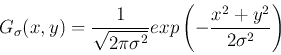
As Laplace operator may detect edges as well as noise (isolated, out-of-range), it may be desirable to smooth the image first by a convolution with a Gaussian kernel of width $\sigma$

$$G_{\sigma}(x,y)=\frac{1}{\sqrt{2\pi\sigma^2}}exp\left(-\frac{x^2+y^2}{2\sigma^2}\right)$$

to suppress the noise before using Laplace for edge detection:

$$\bigtriangleup[G_{\sigma}(x,y) * f(x,y)]=[\bigtriangleup G_{\sigma}(x,y)] * f(x,y)=LoG*f(x,y)$$

The first equal sign is due to the fact that

$$\frac{d}{dt}[h(t)*f(t)]=\frac{d}{dt} \int f(\tau) h(t-\tau)d\... ...int f(\tau) \frac{d}{dt} h(t-\tau)d\tau=f(t)*\frac{d}{dt} h(t)$$

So we can obtain the Laplacian of Gaussian $\bigtriangleup G_{\sigma}(x,y)$ first and then convolve it with the input image. To do so, first consider

$$\frac{\partial}{\partial x} G_{\sigma}(x,y) =\frac{\partia... ...+y^2)/2\sigma^2} =-\frac{x}{\sigma^2}e^{-(x^2+y^2)/2\sigma^2}$$

and

$$\frac{\partial^2}{\partial^2 x} G_{\sigma}(x,y) =\frac{x^2... ...gma^2} =\frac{x^2-\sigma^2}{\sigma^4}e^{-(x^2+y^2)/2\sigma^2}$$

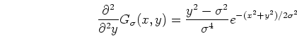
Note that for simplicity we omitted the normalizing coefficient $1/\sqrt{2\pi \sigma^2}$. Similarly we can get

$$\frac{\partial^2}{\partial^2 y} G_{\sigma}(x,y) =\frac{y^2-\sigma^2}{\sigma^4}e^{-(x^2+y^2)/2\sigma^2}$$

Now we have LoG as an operator or convolution kernel defined as

$$LoG \stackrel{\triangle}{=}\bigtriangleup G_{\sigma}(x,y)=\f... ...) =\frac{x^2+y^2-2\sigma^2}{\sigma^4}e^{-(x^2+y^2)/2\sigma^2}$$

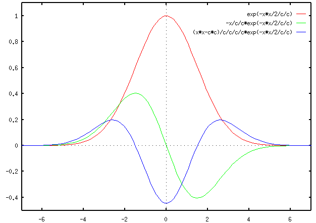
The Gaussian $G(x,y)$ and its first and second derivatives $G'(x,y)$ and $\bigtriangleup G(x,y)$ are shown here:

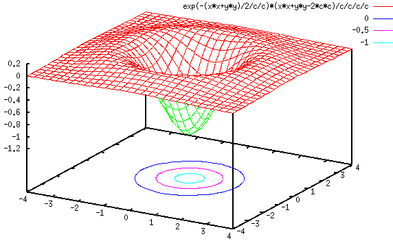
This 2-D LoG can be approximated by a 5 by 5 convolution kernel such as

$$\left[ \begin{array}{ccccc} 0 & 0 & 1 & 0 & 0 \\ 0 & 1 &... ... 0 & 1 & 2 & 1 & 0 \\ 0 & 0 & 1 & 0 & 0 \end{array} \right]$$

The kernel of any other sizes can be obtained by approximating the continuous expression of LoG given above. However, make sure that the sum (or average) of all elements of the kernel has to be zero (similar to the Laplace kernel) so that the convolution result of a homogeneous regions is always zero.

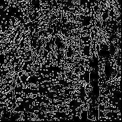
The edges in the image can be obtained by these steps:

• Applying LoG to the image
• Detection of zero-crossings in the image
• Threshold the zero-crossings to keep only those strong ones (large difference between the positive maximum and the negative minimum)

The last step is needed to suppress the weak zero-crossings most likely caused by noise.