Vector form of 1D-DFT

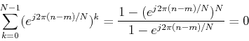
The summation expression for DFT

$$X[n]=\frac{1}{\sqrt{N}}\sum_{m=0}^{N-1} x[m]e^{-mn j2\pi/N} ... ...0}^{N-1} X[n]e^{mn j2\pi/N} =\sum_{n=0}^{N-1} w_N^{-mn} X[n]$$

$$m,n=0, 1, \cdots, N-1$$

can also be written more conveniently as a matrix-vector multiplication:

$$\left[ \begin{array}{c} X[0] . . X[N-1] \end{array} \r... ...t[ \begin{array}{c} x[0] . . x[N-1] \end{array} \right]$$

and

$$\left[ \begin{array}{c} x[0] . . x[N-1] \end{array} \r... ...t[ \begin{array}{c} X[0] . . X[N-1] \end{array} \right]$$

It is obvious that the complexity of 1D DFT takes is $O(N^2)$, which, as we will see later, can be reduced to $O(N\; log_2 N)$ by Fast Fourier Transform (FFT) algorithms.

These matrix-vector multiplications can be represented more concisely as:

$${\bf X}={\bf W}^{-1} {\bf x}$$

and

$${\bf x}={\bf W} {\bf X}$$

where both ${\bf X}$ and ${\bf x}$ are $N \times 1$ column (vertical) vectors:

$${\bf X}\stackrel{\triangle}{=} \left[ \begin{array}{c} X[0] ... ...y}{c} x[0] . . x[N-1] \end{array} \right]_{N\times 1}$$

and $W$ is an $N \times N$ matrix:

$${\bf W}=\left[ \begin{array}{ccc} . & . & . . & w_{mn} & . \\ . & . & . \end{array} \right]_{N\times N}$$

where $w_{mn}$ is an element in the mth row and nth column of matrix $W$ and $w_{mn}^*$ is its complex conjugate:

$$w_{mn}\stackrel{\triangle}{=}\frac{1}{\sqrt{N}}(e^{j2\pi/N})^... ...\;\;\;\;\;\;\; w_{mn}^*=\frac{1}{\sqrt{N}}(e^{-j2\pi/N})^{mn}$$

Obviously ${\bf W}$ is symmetric ($w_{mn}=w_{nm}$)

$${\bf W}^T={\bf W}$$

but ${\bf W}$ is not Hermitian:

$${\bf W}^{*T}={\bf W}^*\neq {\bf W}$$

${\bf W}$ is a unitary matrix,

$${\bf W}^{*T}={\bf W}^*={\bf W}^{-1}$$

because its rows (or columns) are orthogonal:

$$({\bf w}_m, {\bf w}_n)=\sum_{k=0}^{N-1} w_{mk}^* w_{nk} =\fr... ...{k=0}^{N-1} (e^{j2\pi/N})^{(n-m)k} \stackrel{*}{=}\delta_{mn}$$

This is because:

• If $m=n$, $e^{j2\pi/N})^{(n-m)k}=1$ and $({\bf w}_m, {\bf w}_n)=1$
• If $m\ne n$, the summation becomes:
  
  $$\sum_{k=0}^{N-1} (e^{j2\pi(n-m)/N})^k=\frac{1-(e^{j2\pi(n-m)/N})^N}{1-e^{j2\pi(n-m)/N}}=0$$
  
  

The DFT pair can be rewritten as:

$${\bf X}={\bf W}^* {\bf x},\;\;\;\;\;\;\;{\bf x}={\bf W} {\bf X}$$

See additional geometric explanation of unitary/orthogonal transform.