Spectrum Centralization

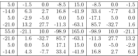
From the previous example, we see that the high frequency components are around the middle part of the 2D spectrum array, while the low frequency components are around the edges of the array. For example, the DC component is at the upper-left corner. Sometime it is preferable to centralize the spectrum so that the DC component and the low frequency components are in the middle of the spectrum array, and high frequency components are around the edges.

Consider a N-point 1D DFT first. Centralization of the 1D spectrum is the same as a shift of the spectrum $X[n]$ by $N/2$ points to either left or right (as $X[n]=X[n+N]$ is periodic, the direction of shift does not matter):

$$X'[n]=X[n-N/2]$$

which can be directly obtained from the time signal $x[m]$ by the shift property of the Fourier transform. Consider the inverse FT of $X[n+\nu]$:

$${\cal F}^{-1}[ X[n-\nu]] = \sum_{n=0}^{N-1}X[n-\nu]e^{j2\pi mn/N} =\sum_{n'=0}^{N-1}X[n']e^{j2\pi (n'+\nu)m/N}$$

$$= \sum_{n'=0}^{N-1}X[n']e^{j2\pi n'm/N}e^{j\pi \nu}=x[m]e^{j2\pi m\nu/N}$$

Here we have assumed $n'=n-\nu$. In particular, when $\nu=N/2$, we have

$${\cal F}^{-1}[X[n-N/2]]=x[m]e^{j2\pi mN/2N}=x[m]e^{j\pi m}=x[m](-1)^m$$

If we change the sign of every other time sample, the corresponding Fourier spectrum will be centralized with DC component in the middle of the 1D array.

Similarly the 2D DFT of a N by N 2D array of spatial samples also has the space shift property:

$${\cal F}{-1}[X[m-N/2,n-N/2]]=x[m,n]e^{j\pi(m+n)}=x[m,n](-1)^{m+n}$$

In other words, if we change the sign of any spatial sample point $x[m,n]$ if $m+n$ is an odd number, i.e.

$$\left[ \begin{array}{rrrr} x[0,0] & -x[0,1] & x[0,2] & \cd... ...ots \\ \vdots & \vdots & \vdots & \ddots \end{array} \right]$$

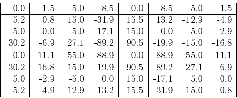
then the resulting 2D Fourier spectrum will be centralized with DC component in the middle and high frequency components around the four edges. For the example above, the real part of the centralized spectrum becomes

$$\begin{tabular}{\vert r\vert rrr\vert r\vert rrr\vert} \hline... ... -7.7 & 33.4 &-41.9 & 16.8 & 2.7 & 6.3 \ \hline \end{tabular}$$

and the imaginary part is:

$$\begin{tabular}{\vert r\vert rrr\vert r\vert rrr\vert} \hline... ... & -13.2 & -15.5 & 31.9 & -15.0 & -0.8 \ \hline \end{tabular}$$