The convolution of two continuous signals ![]() and
and ![]() is defined as
is defined as
Convolution in discrete form is
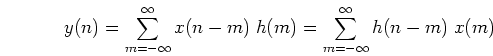
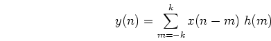
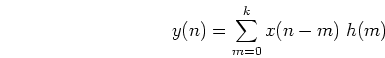
If the system in question were a causal system in time domain, i.e.,
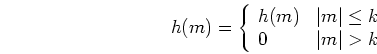
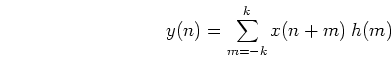
If ![]() is symmetric (almost always true in image processing), i.e.,
is symmetric (almost always true in image processing), i.e.,
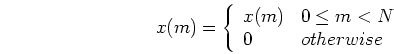
If the input ![]() is finite (always true in reality), i.e.,
is finite (always true in reality), i.e.,
Digital convolution can be best understood graphically (where the index
of ![]() is rearranged).
is rearranged).
Assume the dimensionality of the input signal ![]() is
is ![]() and that of the
kernel
and that of the
kernel ![]() is
is ![]() (usually an odd number), then the dimensionality of
the resulting convolution
(usually an odd number), then the dimensionality of
the resulting convolution ![]() is
is ![]() . However, as it is usually
desirable for the output
. However, as it is usually
desirable for the output ![]() to have the same dimensionality as the input
to have the same dimensionality as the input
![]() ,
, ![]() components at each end of
components at each end of ![]() are dropped. A code segment for this
1D convolution
are dropped. A code segment for this
1D convolution ![]() is given below.
is given below.
![\begin{displaymath}
\par
k=(M-1)/2;
\par
\;\;for (n=0;\; n<N; \; n++) \{
\par
\;...
...par
\;\;\;\;\;\;\;\;\;\;y[n]+=x[n+m]*h[m+k];
\par
\;\; \}
\par
\end{displaymath}](img35.png)
In particular, if the elements of the kernel are all the same (an average or low-pass filter), the we can speed up the convolution process while sliding the kernel over the input signal by taking care of only the two ends of the kernel.
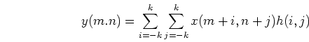
In image processing, all of the discussions above for one-dimensional
convolution are generalized into two dimensions, and ![]() is called a
convolution kernel, or mask.
is called a
convolution kernel, or mask.